Tape-Measure Bias Estimation — Finding a Hidden Offset
“Can we recover a constant tape-bias automatically instead of hand-deriving the arithmetic mean?”
Example adapted from Building and Solving Probabilistic Instrument Models with CaliPy
(Jemil Avers Butt, JISDM 2025, Karlsruhe) DOI: 10.5445/IR/1000179733
What you’ll learn
How to encode the Gaussian model (y\sim\mathcal N(\mu-\theta,\sigma)) in CaliPy
How SVI reproduces the closed-form Least-Squares estimator for (\theta)
How dimension-aware nodes shrink boiler-plate in even the simplest model
1 Background — Why Bias Matters
A steel tape often reads too short or too long by a fixed amount (\theta). When you measure a rod of known length (\mu) (Fig. 1), each observation deviates by that unknown bias plus random noise (\varepsilon):
[ \boxed{y = \mu - \theta + \varepsilon},\qquad \varepsilon\sim\mathcal N(0,\sigma). ]
Classically you solve
(\hat\theta = \tfrac1n\sum_{k=1}^n(\mu - y_k)) by hand
(eq. (1) in the paper).
CaliPy lets us phrase exactly that likelihood and let SVI return the
same answer automatically.
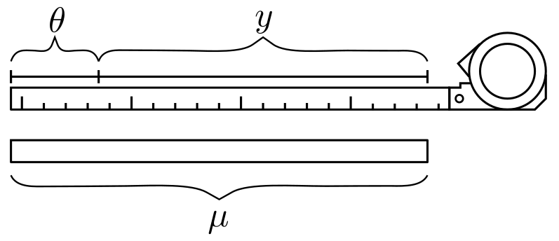
Figure 1 — Schematic tape measurement with unknown bias (\theta). Figure taken from the paper by Butt(2025).
2 Implementation — 12 Lines to a Probabilistic Model
2.1 Dimensions & Nodes
Component |
CaliPy class |
Shape (batch × param) |
|---|---|---|
Bias (\theta) |
|
(n_\text{obs} \times 1) |
Gaussian noise |
|
(n_\text{obs} \times 1) |
n_obs   = 20
batch   = dim_assignment(['obs'], [n_obs])   # i.i.d. samples
scalar  = dim_assignment(['_'],    [])       # empty (=param axis)

# unknown bias θ
θ_ns = NodeStructure(UnknownParameter)
θ_ns.set_dims(batch_dims=batch, param_dims=scalar)
θ     = UnknownParameter(θ_ns, name='theta')

# noise wrapper  𝒩(mean, σ)
noise_ns = NodeStructure(NoiseAddition)
noise_ns.set_dims(batch_dims=batch, event_dims=scalar)
noise = NoiseAddition(noise_ns)
2.2 Forward Model
class TapeBiasProbModel(CalipyProbModel):
    def model(self, _, observations=None):
        θ_val = θ.forward()                       # shape (n_obs,)
        mean  = mu_true - θ_val
        out   = noise.forward({'mean': mean,
                               'standard_deviation': sigma_true},
                              observations)
        return out
No manual plates, broadcasting, or log-prob math required.
3 Running Inference
probmodel = TapeBiasProbModel()

y_obs = CalipyTensor(data, dims=batch)          # simulated data
elbo = probmodel.train(None, y_obs,
                       optim_opts=dict(optimizer = pyro.optim.NAdam({"lr":0.01}),
                                       loss      = pyro.infer.Trace_ELBO(),
                                       n_steps   = 1_000))
4 Results
Node_1__param_theta
 tensor(0.0103, requires_grad=True)
True θ     : 0.0100
Empirical  : 0.0101   # arithmetic mean (LS)

Figure 2 — ELBO converges smoothly to the global optimum.
Take-aways
SVI = LS for a linear-Gaussian one-parameter model — check.
Declaring
UnknownParameterremoved all algebra from eq. (1).The same scaffold scales to heteroscedastic σ or priors in one line.
5 Key Insights
Declarative ≠ verbose – this entire example uses < 40 lines of actual model code.
Dimension-aware tensors keep sample shapes and math symbols in sync.
Swap-in inference – change
Trace_ELBOtoNUTSand you immediately get MCMC draws.
6 Next Steps
Make (\sigma) an
UnknownVarianceand learn it too.Give (\theta) a Gaussian prior centred at the manufacturer’s spec.
Simulate 10 000 observations and try sub-batch SVI.
7 Full Code
#!/usr/bin/env python3
# -*- coding: utf-8 -*-
"""
The goal of this script is to employ calipy to model a simple tape measure bias
estimation problem as dealt with in section 4.1 of the paper: "Building and Solving
Probabilistic Instrument Models with CaliPy" presented at JISDM 2025. The overall
measurement process consists in gathering length measurements y of an object with
length mu effected by a bias theta; the corresponding probabilistic model is given
as y ~N(mu - theta, sigma) where N is the Gaussian distribution. Here mu and sigma
are assumed known, y is observed, and theta is to be inferred.
We want to infer theta from observations y without performing any further manual
computations.
For this, do the following:
    1. Imports and definitions
    2. Simulate some data
    3. Load and customize effects
    4. Build the probmodel
    5. Perform inference
    6. Analyse results and illustrate

The script is meant solely for educational and illustrative purposes. Written by
Dr. Jemil Avers Butt, Atlas optimization GmbH, www.atlasoptimization.com.
"""


"""
    1. Imports and definitions
"""


# i) Imports

# base packages
import torch
import pyro
import matplotlib.pyplot as plt

# calipy
import calipy
from calipy.core.base import NodeStructure, CalipyProbModel
from calipy.core.effects import UnknownParameter, NoiseAddition
from calipy.core.utils import dim_assignment
from calipy.core.tensor import CalipyTensor


# ii) Definitions

n_meas = 20


"""
    2. Simulate some data
"""


# i) Set up sample distributions

theta_true = 0.01
mu_true = torch.tensor(1.0)
sigma_true = torch.tensor(0.1)


# ii) Sample from distributions

data_distribution = pyro.distributions.Normal(mu_true - theta_true, sigma_true)
data = data_distribution.sample([n_meas])

# The data now is a tensor of shape [n_meas] and reflects biased measurements being
# taken of a single object of length mu with a single tape measure.

# We now consider the data to be an outcome of measurement of some real world
# object; consider the true underlying data generation process to be unknown
# from now on.


"""
    3. Load and customize effects
"""


# i) Set up dimensions

batch_dims = dim_assignment(['bd_1'], dim_sizes = [n_meas])
event_dims = dim_assignment(['ed_1'], dim_sizes = [])
param_dims = dim_assignment(['pd_1'], dim_sizes = [])


# ii) Set up dimensions for mean parameter mu

# Setting up requires correctly specifying a NodeStructure object. You can get
# a template for the node_structure by calling generate_template() on the example
# node_structure delivered with the class description. Here, we call the example
# node structure, then set the dims; required dims that need to be provided can
# be found via help(mu_ns.set_dims).

# theta setup
theta_ns = NodeStructure(UnknownParameter)
theta_ns.set_dims(batch_dims = batch_dims, param_dims = param_dims,)
theta_object = UnknownParameter(theta_ns, name = 'theta')


# iii) Set up the dimensions for noise addition
# This requires again the batch shapes and event shapes. They are used to set
# up the dimensions in which the noise is i.i.d. and the dims in which it is
# copied. Again, required keys can be found via help(noise_ns.set_dims).
noise_ns = NodeStructure(NoiseAddition)
noise_ns.set_dims(batch_dims = batch_dims, event_dims = event_dims)
noise_object = NoiseAddition(noise_ns, name = 'noise')


"""
    4. Build the probmodel
"""


# i) Define the probmodel class

class DemoProbModel(CalipyProbModel):
    def __init__(self, **kwargs):
        super().__init__(**kwargs)

        # integrate nodes
        self.theta_object = theta_object
        self.noise_object = noise_object

    # Define model by forward passing
    def model(self, input_vars = None, observations = None):
        theta = self.theta_object.forward()

        inputs = {'mean':mu_true - theta, 'standard_deviation': sigma_true}
        output = self.noise_object.forward(input_vars = inputs,
                                           observations = observations)

        return output

    # Define guide (trivial since no posteriors)
    def guide(self, input_vars = None, observations = None):
        pass

demo_probmodel = DemoProbModel()


"""
    5. Perform inference
"""


# i) Set up optimization

adam = pyro.optim.NAdam({"lr": 0.01})
elbo = pyro.infer.Trace_ELBO()
n_steps = 1000

optim_opts = {'optimizer': adam, 'loss' : elbo, 'n_steps': n_steps}


# ii) Train the model

input_data = None
data_cp = CalipyTensor(data, dims = batch_dims + event_dims)
optim_results = demo_probmodel.train(input_data, data_cp, optim_opts = optim_opts)


"""
    6. Analyse results and illustrate
"""


# i)  Plot loss

plt.figure(1, dpi = 300)
plt.plot(optim_results)
plt.title('ELBO loss')
plt.xlabel('epoch')

# ii) Print  parameters

for param, value in pyro.get_param_store().items():
    print(param, '\n', value)

print('True values of theta = ', theta_true)
print('Results of taking empirical means for theta = ', mu_true - torch.mean(data))