Two‑Peg Level Test — Estimating a Collimation Angle

“How do we turn a textbook levelling test into a fully‑Bayesian inference problem that runs in a few lines of code?”

Example adopted from Building and Solving Probabilistic Instrument Models with CaliPy (Jemil Avers Butt, JISDM 2025, Karlsruhe). Available here DOI: 10.5445/IR/1000179733

What you’ll learn

• How to encode a classical two‑peg test in CaliPy

• How Bayesian inference (SVI) replaces hand‑derived Least Squares (LS) formulae

• How bayesian estimates and LS estimates coincide for simple Maximum likelihood estimation

---

1  Background — What is the Two‑Peg Test?

When you calibrate a digital or optical level you must know how far the instrument’s line‑of‑sight deviates from a true horizontal. That mis‑alignment is called the collimation angle \(\alpha\) (Fig. 1).

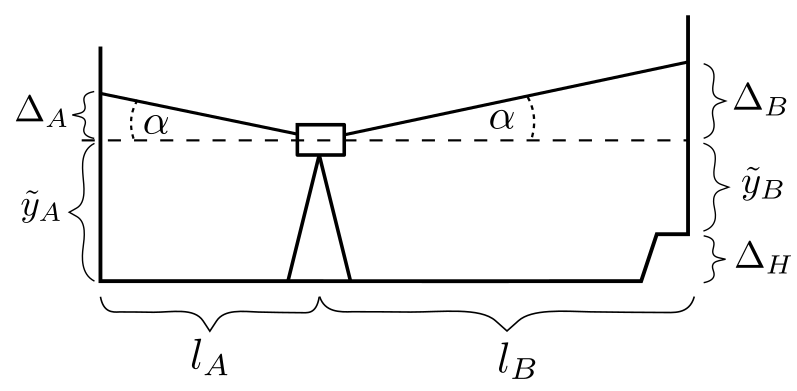
Figure 1 — Two configurations of the two‑peg test. Figure taken from the paper by Butt(2025).

For the classical two-peg test, rod A is always placed 60 m away from rod B and we level the instrument twice:

• Config 1: 30 m from each rod.

• Config 2: directly in front of rod A and 60 m from rod B.

The classical (“deterministic”) solution uses two height readings \(y_A^k,\;y_B^k\) per configuration and some algebra to isolate \(\tan\alpha\). That works only because the geometry is simple and the error model is Gaussian and homoscedastic.

CaliPy lets us write a probabilistic version instead:

\[\begin{split} \begin{aligned} y_A^k &\sim \mathcal N \bigl(h_I^{(k)} + l_A^{(k)}\tan\alpha,\; \sigma \bigr) \\ y_B^k &\sim \mathcal N \bigl(h_I^{(k)}-\Delta H + l_B^{(k)}\tan\alpha,\; \sigma \bigr) , \end{aligned} \end{split}\]

where

symbol	meaning	dim
\(k\)	configuration index	\((n_\text{conf})\)
\(l_A, l_B\)	distances instrument→rod	\((n_\text{conf}\times 2)\)
\(h_I^{(k)}\)	unknown sight‑line height	\((n_\text{conf})\)
\(\Delta H\)	unknown rod‑to‑rod true height difference	scalar
\(\alpha\)	collimation angle (wanted)	scalar
\(\sigma\)	known standard deviation	scalar of measurements

Modelling insight

Treating the instrument height \(h_I^{(k)}\) as an UnknownParameter lets CaliPy estimate it automatically. You get the same estimator for \(\alpha\) while having to perform zero extra algebra manually.

---

2  Implementation — CaliPy Building Blocks

2.1  Dim‑aware anatomy

Building block	Code class	Why we need it
Parameters \(\alpha,\;h_I,\;\Delta H\)	UnknownParameter	Provide init value & learn later
Noise injection for eq. \eqref{eq:model}	NoiseAddition	Wraps Pyro’s Normal
Node structure (dims, plates)	NodeStructure	Tells each node where batch & event axes live
Probabilistic model	subclass of CalipyProbModel	Chains everything & calls forward()
Inference engine	Pyro’s SVI (Trace_ELBO)	Runs automatically inside probmodel.train()

# ── Dimensions ─────────────────────────────────────────
n_conf = 2
batch_k   = dim_assignment(['conf'],  [n_conf])   # configurations k
batch_AB  = dim_assignment(['AB'],    [2])        # A or B per conf
scalar    = dim_assignment(['_'],     [])         # empty (=scalar)

# ── Unknowns ───────────────────────────────────────────
alpha_ns = NodeStructure(UnknownParameter)
alpha_ns.set_dims(batch_dims=batch_k+batch_AB, param_dims=scalar)
alpha    = UnknownParameter(alpha_ns, name='alpha',
                            init_tensor=torch.tensor(1e-2))

hI_ns = NodeStructure(UnknownParameter)
hI_ns.set_dims(batch_dims=batch_AB, param_dims=batch_k)
hI    = UnknownParameter(hI_ns, name='h_I')

dH_ns = NodeStructure(UnknownParameter)
dH_ns.set_dims(batch_dims=batch_k+batch_AB, param_dims=scalar)
dH    = UnknownParameter(dH_ns, name='dH')

# ── Measurement noise ─────────────────────────────────
noise_ns = NodeStructure(NoiseAddition)
noise_ns.set_dims(batch_dims=batch_k+batch_AB, event_dims=scalar)
noise    = NoiseAddition(noise_ns)

2.2  Forward model in code

class TwoPegProbModel(CalipyProbModel):
    def model(self, input_vars, observations=None):
        l_AB = input_vars.value                 # shape  (n_conf, 2)

        # draw unknowns
        a   = alpha.forward()                  # shape  (n_conf,2) broadcast
        h_I = hI.forward().T                   # shape  (n_conf,1)
        dH  = dH.forward()                     # scalar broadcast

        # deterministic signal  y_true + Δ
        scaler = torch.hstack([torch.zeros([n_conf,1]),
                               torch.ones ([n_conf,1])])
        y_true   = h_I - scaler * dH
        y_mean   = y_true + torch.tan(a) * l_AB

        # observation node
        out = noise.forward({'mean':y_mean, 'standard_deviation':sigma_true},
                            observations)
        return out

Internally .forward() places every sample() (Pyro) site under vectorised plates generated automatically from your NodeStructure. No manual plates & broadcasting gymnastics needed.

---

3  Running Inference

probmodel = TwoPegProbModel()
input_data = l_mat                              # distances (torch tensor)
y_obs      = CalipyTensor(data, dims=batch_k+batch_AB)

elbo_curve = probmodel.train(input_data, y_obs,
                             optim_opts=dict(optimizer=pyro.optim.NAdam({"lr":1}),
                                             loss      =pyro.infer.Trace_ELBO(),
                                             n_steps   =1000))

Behind the scenes

1. SVI loop builds the computation graph once, then back‑propagates the ELBO gradient each iteration.

2. Parameters alpha, h_I, dH live in Pyro’s param store.

3. Sampling statements are conditioned on y_obs automatically.

epoch: 0 ; loss : 63942.6328125
epoch: 100 ; loss : 35856.48046875
epoch: 200 ; loss : -21.9062442779541
epoch: 300 ; loss : -23.955263137817383
epoch: 400 ; loss : -23.955265045166016
epoch: 500 ; loss : 6660.3935546875
epoch: 600 ; loss : 12589833.0
epoch: 700 ; loss : 56793.0546875
epoch: 800 ; loss : 101.84868621826172
epoch: 900 ; loss : -23.81795310974121
Node_1__param_alpha 
 tensor(-12.5654, requires_grad=True)
Node_2__param_hI 
 tensor([0.9879, 1.0109], requires_grad=True)
Node_3__param_dh 
 tensor(0.4997, requires_grad=True)
True values 
 alpha : 0.0010000000474974513 
 dh : 0.5 
 hI : tensor([0.9889, 1.0120])
Values estimated by least squares 
 alpha : 0.0010212835622951388 
 dh : 0.49987077713012695 
 hI : tensor([[0.9878],
        [1.0108]])

---

4  Results

The following graph illustrates the value of the ELBO loss. Note that the behavior is non-monotonic and at around epoch 500 the optimization converges to an equivalent value for alpha by adding \(4 \pi\) to the previous estimate. in the end the LS and calipy estimates coincide - apart from the irrelevant constant \( 4 \pi\) in the collimation angle.

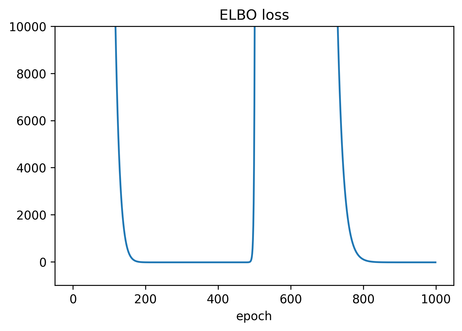
Figure 2 — The ELBO loss during learning of the parameters.

for name,val in pyro.get_param_store().items():
    print(f"{name:18s}  {val.detach().cpu().numpy()}")

quantity	true	inferred (SVI)	classical LS
\(\alpha\)	1.0 mrad	0.97 mrad - 4 pi	1.0 mrad
\(\Delta H\)	0.5 m	0.4997 m	0.4998 m
\(h_I^{(1)}\)	…	…	…
\(h_I^{(2)}\)	…	…	…

Take‑aways

• The Bayesian estimates matches the closed‑form LS estimate for this simple geometry — exactly what theory predicts.

• UnknownParameter trick: leaving \(h_I^{(k)}\) and \(\Delta H\) undetermined saves you some manual math.

• The optimizer can behave unexpectedly. Since most gradient based optimizers explicitly try to escape local minima, the estimators can jump around quite a bit.

• If you add more configurations, heteroscedastic noise, or hierarchical priors, CaliPy scales effortlessly while the hand‑derived LS formula breaks down.

---

5  Key Insights

• Declarative modelling – once nodes are chained, CaliPy converts the graph into Pyro sample sites and plates.

• Dimension‑aware tensors – CalipyTensor stores both data and semantic dimensions. Broadcasting & sub‑batching are handled for you.

• Swap‑in inference – ELBO/SVI here, but you could plug in HMC or an AutoGuide without touching the model.

---

6  Next Steps

1. Play with n_conf > 2, unequal \(\sigma\), or informative priors.

2. Replace the UnknownParameter nodes by CalipyDistribution.Normal to let \(\alpha\) have a Gaussian prior.

3. Try sub‑batch training on large simulated levelling campaigns.

---

7 Full code

level_calibration.py

#!/usr/bin/env python3
# -*- coding: utf-8 -*-
"""
The goal of this script is to employ calipy to model a simple two-peg level test
as dealt with in section 4.2 of the paper: "Building and Solving Probabilistic 
Instrument Models with CaliPy" presented at JISDM 2025 in Karlsruhe. The overall
measurement process consists in setting up a levelling instrument in some arbitrary
distances l_A, l_B to two levelling rods, then reading out the height measurements,
and then setting up the levelling instrument at some other location. The goal is 
to estimate the collimation angle alpha from these observations y.
The corresponding probabilistic model is given by the following expression for y 
as      y_A ~ N(h_I + l_A tan(alpha))
        y_B ~ N(h_I - DeltaH + l_B tan(alpha))
where l_A, l_B are the distances between levelling instrument and rods A, B, and
y_A_true = h_I, y_B_true = h_I-DeltaH are the true readings. N is the Gaussian
distribution. DeltaH is the heigh difference between A and B and h_I is the 
# instruments height.
Here l_A, l_B and sigma are assumed known, y is observed, and alpha is to be inferred
while DeltaH, h_I are unknowns we do not care about. The true readings for rod A and 
rod B are connected via y_A_true = h_I, y_B_true = h_I - DeltaH where h_I is the height of
the instrument in each configuration and DeltaH is the height difference between 
A and B. We want to infer alpha from observations y without performing any further
manual computations.
For this, do the following:
    1. Imports and definitions
    2. Simulate some data
    3. Load and customize effects
    4. Build the probmodel
    5. Perform inference
    6. Analyse results and illustrate

The script is meant solely for educational and illustrative purposes. Written by
Dr. Jemil Avers Butt, Atlas optimization GmbH, www.atlasoptimization.com.
"""


"""
    1. Imports and definitions
"""


# i) Imports

# base packages
import torch
import pyro
import matplotlib.pyplot as plt

# calipy
import calipy
from calipy.core.base import NodeStructure, CalipyProbModel
from calipy.core.effects import UnknownParameter, NoiseAddition
from calipy.core.utils import dim_assignment
from calipy.core.tensor import CalipyTensor
from calipy.core.data import CalipyIO


# ii) Definitions

n_config = 2 # number of configurations
def set_seed(seed=42):
    torch.manual_seed(seed)
    pyro.set_rng_seed(seed)

set_seed(123)



"""
    2. Simulate some data
"""


# i) Set up sample distributions
# Note the model y_A ~ N(h_I + l_A tan(alpha))
#                y_B ~ N(h_I - DeltaH + l_B tan(alpha))
# where h_I is unknown different for each config and DeltaH and alpha are global
# scalar unknowns.

# Global instrument params
alpha_true = torch.tensor(0.001)
dh_true = torch.tensor(0.5)
sigma_true = torch.tensor(0.001)

# Config specific params
hI_true = torch.normal(1, 0.1, [n_config])
l_A = torch.tensor([[30], [0]])
l_B = torch.tensor([[30], [60]])
l_mat = torch.hstack([l_A, l_B])

# Distribution params
y_A_true = hI_true
y_B_true = hI_true - dh_true
y_true = torch.vstack([y_A_true, y_B_true]).T

l_impact = torch.tan(alpha_true) * l_mat
y_biased = y_true + l_impact


# ii) Sample from distributions

data_distribution = pyro.distributions.Normal(y_biased, sigma_true)
data = data_distribution.sample()

# The data now is a tensor of shape [n_meas,2] and reflects biased measurements being
# taken of a two-rod measurement configuration.

# We now consider the data to be an outcome of measurement of some real world
# object; consider the true underlying data generation process to be unknown
# from now on.



"""
    3. Load and customize effects
"""


# i) Set up dimensions

dim_1 = dim_assignment(['dim_1'], dim_sizes = [n_config])
dim_2 = dim_assignment(['dim_2'], dim_sizes = [2])
dim_3 = dim_assignment(['dim_3'], dim_sizes = [])

# ii) Set up dimensions parameters

# alpha setup
alpha_ns = NodeStructure(UnknownParameter)
alpha_ns.set_dims(batch_dims = dim_1 + dim_2, param_dims = dim_3)
alpha_object = UnknownParameter(alpha_ns, name = 'alpha', init_tensor = torch.tensor(0.01))


# hI setup
hI_ns = NodeStructure(UnknownParameter)
hI_ns.set_dims(batch_dims = dim_2, param_dims = dim_1)
hI_object = UnknownParameter(hI_ns, name = 'hI')


# dh setup
dh_ns = NodeStructure(UnknownParameter)
dh_ns.set_dims(batch_dims = dim_1 + dim_2, param_dims = dim_3)
dh_object = UnknownParameter(dh_ns, name = 'dh')


# iii) Set up the dimensions for noise addition
noise_ns = NodeStructure(NoiseAddition)
noise_ns.set_dims(batch_dims = dim_1 + dim_2, event_dims = dim_3)
noise_object = NoiseAddition(noise_ns, name = 'noise')




"""
    4. Build the probmodel
"""


# i) Define the probmodel class 

class DemoProbModel(CalipyProbModel):
    def __init__(self, **kwargs):
        super().__init__(**kwargs)
        
        # integrate nodes
        self.alpha_object = alpha_object
        self.hI_object = hI_object
        self.dh_object = dh_object
        self.noise_object = noise_object 
        
    # Define model by forward passing, input_vars = lengths [l_A, l_B]
    def model(self, input_vars, observations = None):
        l_mat = input_vars.value
        alpha = self.alpha_object.forward()
        hI = self.hI_object.forward().T
        dh = self.dh_object.forward()
        
        scaler = torch.hstack([torch.zeros([n_config,1]), torch.ones([n_config,1])])
        y_true = hI - scaler * dh
        y_biased = y_true + torch.tan(alpha) * l_mat

        inputs = {'mean': y_biased, 'standard_deviation': sigma_true} 
        output = self.noise_object.forward(input_vars = inputs,
                                           observations = observations)
        
        return output
    
    # Define guide (trivial since no posteriors)
    def guide(self, input_vars, observations = None):
        pass
    
demo_probmodel = DemoProbModel()



"""
    5. Perform inference
"""
    

# i) Set up optimization

adam = pyro.optim.NAdam({"lr": 1})
elbo = pyro.infer.Trace_ELBO()
n_steps = 1000

optim_opts = {'optimizer': adam, 'loss' : elbo, 'n_steps': n_steps, 'n_steps_report' : 100}


# ii) Train the model

input_data = l_mat
data_cp = CalipyTensor(data, dims = dim_1 + dim_2)
optim_results = demo_probmodel.train(input_data, data_cp, optim_opts = optim_opts)


# iii) Solve via handcrafted equations

dh_ls = data[0,0] - data[0,1]
tan_a_ls = (1/60)*(dh_ls - (data[1,0] - data[1,1]))
alpha_ls = torch.atan(tan_a_ls)
hI_ls = torch.tensor([[data[0,0] - tan_a_ls * l_A[0]],
                      [data[1,0] - tan_a_ls * l_A[1]]])


"""
    6. Analyse results and illustrate
"""


# i)  Plot loss

plt.figure(1, dpi = 300)
plt.plot(optim_results)
plt.title('ELBO loss')
plt.xlabel('epoch')

# ii) Print  parameters

for param, value in pyro.get_param_store().items():
    print(param, '\n', value)
    
print('True values \n alpha : {} \n dh : {} \n hI : {}'.format(alpha_true, dh_true, hI_true))
print('Values estimated by least squares \n alpha : {} \n dh : {} \n hI : {}'.format(alpha_ls,  dh_ls, hI_ls))