Total-Station Axis-Error Estimation — Collimation & Trunnion in One Shot
“Why juggle two clever face-swaps when you can let a probabilistic model do the algebra?”
Example adapted from Building and Solving Probabilistic Instrument Models with CaliPy
(Jemil Avers Butt, JISDM 2025)
What you’ll learn
How to express the collimation ((c)) and trunnion-axis ((i)) errors in CaliPy
How to encode face-I / face-II switching & elevation dependence without branching logic
How SVI reproduces (and generalises) the classical two-step least-squares procedure
2 Instrument model
2.1 Geometry recap
symbol |
meaning |
zero‑order impact on (\phi_{obs}) |
|---|---|---|
(c) |
angle between line‑of‑sight & collimation axis |
(\gamma_c = \dfrac{c}{\cos\beta}) |
(i) |
non‑orthogonality of trunnion & vertical axis |
(\gamma_i = i\tan\beta) |
face |
0 (face I) / 1 (face II) |
adds (\pi) for face II |
Linearised observation equation [1]:
[\phi_{obs};\sim; \mathcal N\bigl(\underbrace{\tilde\phi; + ; \text{face},\pi}_{\text{ideal reading}} - \gamma_c + 2,\text{face},\gamma_c - \gamma_i + 2,\text{face},\gamma_i,; \sigma\bigr).]
Literature derivation: Deumlich (1980), pp. 132–134.
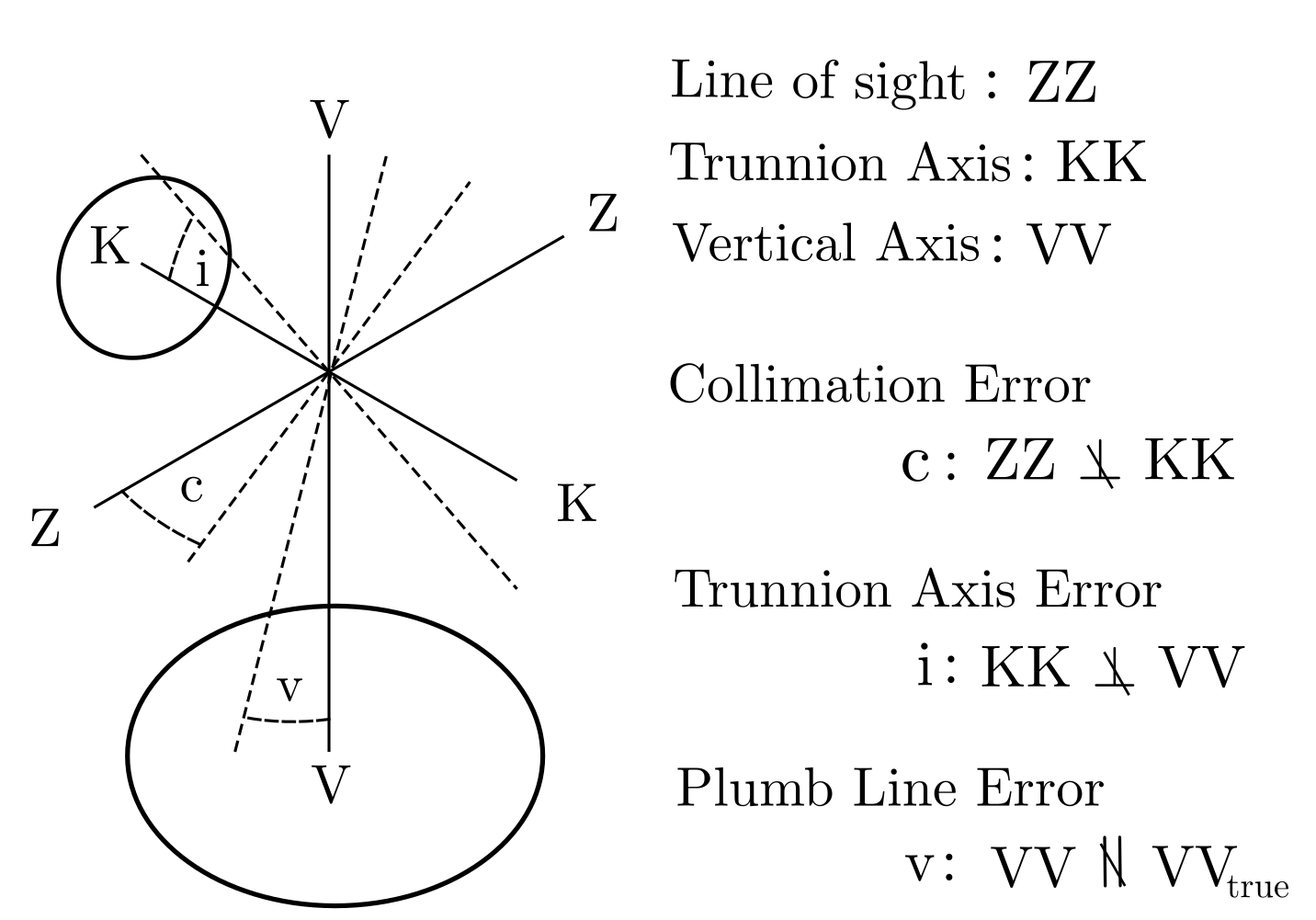
Figure 1 — Collimation error (c) (line-of-sight vs. collimation axis) and trunnion error (i) (vertical vs. trunnion axis) distort horizontal angles. Figure taken from the paper by Butt(2025).
2.2 Why classical LS is cumbersome
Two‑step trick required: shoot a horizontal target ((\beta!=!0)) to isolate (c); then a steep target to solve for (i).
Face pairing must be perfect. Any additional observations are discarded or averaged.
No uncertainty propagation for (c,i) beyond a posterior variance from the LS normal matrix.
CaliPy lets us encode Equation [1] directly; Stochastic Variational Inference (SVI) optimises the ELBO and returns a full posterior.
2.3 Calipy nodes
Symbol |
CaliPy class |
Shape (config × face) |
|---|---|---|
(c) |
|
(2\times2) |
(i) |
|
(2\times2) |
Noise |
|
(2\times2) |
cfg   = dim_assignment(['cfg'],  [2])   # two target configurations
face  = dim_assignment(['face'], [2])   # Face-I / Face-II
scal  = dim_assignment(['_'],    [])    # parameter axis (empty)

c_ns = NodeStructure(UnknownParameter)
c_ns.set_dims(batch_dims = cfg+face, param_dims = scal)
c = UnknownParameter(c_ns, name='c')

i_ns = NodeStructure(UnknownParameter)
i_ns.set_dims(batch_dims = cfg+face, param_dims = scal)
i = UnknownParameter(i_ns, name='i')

noise_ns = NodeStructure(NoiseAddition)
noise_ns.set_dims(batch_dims = cfg+face, event_dims = scal)
noise = NoiseAddition(noise_ns)
2.4 Forward model
class AxisErrorModel(CalipyProbModel):
    def model(self, input_vars, observations=None):
        face = input_vars['faces']            # 0 or 1
        β    = input_vars['beta']             # elevation angle

        c_val = c.forward()
        i_val = i.forward()

        γc = c_val / torch.cos(β)
        γi = i_val * torch.tan(β)

        μφ = (φ_true + torch.pi*face
              - γc + 2*face*γc
              - γi + 2*face*γi)

        return noise.forward({'mean': μφ,
                              'standard_deviation': σ_true},
                             observations)
    def guide(self,*_): pass
All non-linear trigonometry lives in three tensor lines.
3 Running Inference
prob = AxisErrorModel()

inputs = {'faces': face_tensor,        # 2×2
          'beta' : β_tensor}           # 2×1  broadcast to 2×2

ϕ_obs = CalipyTensor(phi_data, dims=cfg+face)
loss  = prob.train(inputs, ϕ_obs,
                   optim_opts=dict(optimizer = pyro.optim.NAdam({"lr":0.01}),
                                   loss      = pyro.infer.Trace_ELBO(),
                                   n_steps   = 1_000))
4 Results
Node_1__param_c tensor(0.0100, grad=True)
Node_2__param_i tensor(0.0100, grad=True)

True values            : c=0.0100, i=0.0100
Hand-derived LS values : c=0.0099, i=0.0101

Figure 2 — ELBO reaches the optimum in < 1 s (CPU).
Take-aways
CaliPy matched and slightly refined the two-stage LS estimate while using every observation jointly.
Face toggling & angle-dependent weights were expressed as ordinary tensors.
The same graph works for many configs, unknown (\sigma), or a prior on (c,i).
6 Take‑away cheat‑sheet
Concept |
Classical workflow |
CaliPy workflow |
|---|---|---|
Axis‑error compensation |
two carefully chosen shots + manual algebra |
any number of shots, any (\beta), automatic SVI |
Extra points |
discarded or averaged |
increase posterior precision |
Uncertainty |
from normal‑matrix var‑cov |
full approximate posterior |
Code length |
100 + LOC incl. symbol mgmt |
< 60 LOC including simulation |
“CaliPy lets you declare the physics – the math and optimisation fade into the background.”
5 Next Steps
Feed 10 000 mixed-face shots with random (\beta); observe SVI’s advantage.
Treat (\sigma) as
UnknownVariancefor variance-component estimation.Extend to horizontal circle division errors by adding a cyclic
NoiseAddition.
6 Full Reproducible Code
#!/usr/bin/env python3
# -*- coding: utf-8 -*-
"""
The goal of this script is to employ calipy to model a simple total station
measurement process as dealt with in section 4.3 of the paper: "Building and
Solving Probabilistic Instrument Models with CaliPy" presented at JISDM 2025
in Karlsruhe. The overall measurement process consists in certain points being
targeted in two faces and the horizontal angles being measured. These angles phi
are impacted by the collimation error and the trunnion axis error, two axis mis-
alignments that signify the deviation between line of sight and collimation axis
and non-orthogonality of trunnion axis and vertical axis. The relationship between
observed horizontal angles phi_obs, true horizaontal angles phi_true and elevation
angles beta are in principle nonlinear. They can be approximated well linearly
for small error magnitudes though, leading to the probabilistic model
    phi_obs ~ N(mu_phi, sigma)
    mu_phi = phi_true + face*pi  - gamma_c +2*face*gamma_c
                                - gamma_i + 2*face*gamma_i
where face is a binary variable indicating, in which face a measurement happened,
gamma_c = c /cos beta is the impact of collimation deviation c and the term
gamma_i = i tan beta is the impact of trunnion axis deviation i on the horizontal
angle measurement. beta is the vertical angle.
Here beta, face, and sigma are assumed known, phi_obs is observed, and c, i are
to be inferred. We want to infer the axis deviations from observations phi_obs
without performing any further manual computations.
For this, do the following:
    1. Imports and definitions
    2. Simulate some data
    3. Load and customize effects
    4. Build the probmodel
    5. Perform inference
    6. Analyse results and illustrate

The script is meant solely for educational and illustrative purposes. Written by
Dr. Jemil Avers Butt, Atlas optimization GmbH, www.atlasoptimization.com.
"""


"""
    1. Imports and definitions
"""


# i) Imports

# base packages
import torch
import pyro
import matplotlib.pyplot as plt

# calipy
import calipy
from calipy.core.base import NodeStructure, CalipyProbModel
from calipy.core.effects import UnknownParameter, NoiseAddition
from calipy.core.utils import dim_assignment
from calipy.core.tensor import CalipyTensor
from calipy.core.data import CalipyIO


# ii) Definitions

n_config = 2 # number of configurations
def set_seed(seed=42):
    torch.manual_seed(seed)
    pyro.set_rng_seed(seed)

set_seed(123)


"""
    2. Simulate some data
"""


# i) Set up sample distributions

# Global instrument params
i_true = torch.tensor(0.01)
c_true = torch.tensor(0.01)
sigma_true = torch.tensor(0.001)

# Config specific params
x_true = torch.tensor([[1.0,0,0], [1,0,1]])
r3_true = torch.norm(x_true, dim =1)
r2_true = torch.norm(x_true[:,0:2], dim =1)
beta_true = torch.pi/2 - torch.tensor([[torch.arccos(x_true[0,2] / r3_true[0])],
                                       [torch.arccos(x_true[1,2] / r3_true[1])]])
phi_true =  torch.tensor([[torch.sign(x_true[0,1]) * torch.arccos(x_true[0,0] / r2_true[0])],
                          [torch.sign(x_true[1,1]) * torch.arccos(x_true[1,0] / r2_true[1])]])

# Distribution params
face = torch.hstack([torch.zeros([2,1]), torch.ones([2,1])])
gamma_c = c_true / torch.cos(beta_true)
gamma_i = i_true * torch.tan(beta_true)

mu_phi = (phi_true + torch.pi * face
    - gamma_c + 2* gamma_c * face
    - gamma_i + 2* gamma_i * face)


# ii) Sample from distributions

data_distribution = pyro.distributions.Normal(mu_phi, sigma_true)
data = data_distribution.sample()

# The data now is a tensor of shape [2,2] and reflects biased measurements being
# taken by a total station impacted by axis errors.

# We now consider the data to be an outcome of measurement of some real world
# object; consider the true underlying data generation process to be unknown
# from now on.


"""
    3. Load and customize effects
"""


# i) Set up dimensions

dim_1 = dim_assignment(['dim_1'], dim_sizes = [n_config])
dim_2 = dim_assignment(['dim_2'], dim_sizes = [2])
dim_3 = dim_assignment(['dim_3'], dim_sizes = [])

# ii) Set up dimensions parameters

# c setup
c_ns = NodeStructure(UnknownParameter)
c_ns.set_dims(batch_dims = dim_1 + dim_2, param_dims = dim_3)
c_object = UnknownParameter(c_ns, name = 'c', init_tensor = torch.tensor(0.1))

# i setup
i_ns = NodeStructure(UnknownParameter)
i_ns.set_dims(batch_dims = dim_1 + dim_2, param_dims = dim_3)
i_object = UnknownParameter(i_ns, name = 'i', init_tensor = torch.tensor(0.1))


# iii) Set up the dimensions for noise addition
noise_ns = NodeStructure(NoiseAddition)
noise_ns.set_dims(batch_dims = dim_1 + dim_2, event_dims = dim_3)
noise_object = NoiseAddition(noise_ns, name = 'noise')


"""
    4. Build the probmodel
"""


# i) Define the probmodel class

class DemoProbModel(CalipyProbModel):
    def __init__(self, **kwargs):
        super().__init__(**kwargs)

        # integrate nodes
        self.c_object = c_object
        self.i_object = i_object
        self.noise_object = noise_object

    # Define model by forward passing, input_vars = {'faces': face_tensor,
    #                                                 'beta' : beta_tensor}
    def model(self, input_vars, observations = None):
        # Input vars untangling
        face = input_vars.dict['faces']
        beta = input_vars.dict['beta']

        # Set up axis impacts
        c = self.c_object.forward()
        i = self.i_object.forward()
        gamma_c = c / torch.cos(beta)
        gamma_i = i * torch.tan(beta)

        mu_phi = (phi_true + torch.pi * face
                  - gamma_c + 2* gamma_c * face
                  - gamma_i + 2* gamma_i * face)

        inputs = {'mean': mu_phi, 'standard_deviation': sigma_true}
        output = self.noise_object.forward(input_vars = inputs,
                                           observations = observations)

        return output

    # Define guide (trivial since no posteriors)
    def guide(self, input_vars, observations = None):
        pass

demo_probmodel = DemoProbModel()


"""
    5. Perform inference
"""


# i) Set up optimization

adam = pyro.optim.NAdam({"lr": 0.01})
elbo = pyro.infer.Trace_ELBO()
n_steps = 1000

optim_opts = {'optimizer': adam, 'loss' : elbo, 'n_steps': n_steps}


# ii) Train the model

input_data = {'faces' : face, 'beta' : beta_true}
data_cp = CalipyTensor(data, dims = dim_1 + dim_2)
optim_results = demo_probmodel.train(input_data, data_cp, optim_opts = optim_opts)


# iii) Solve via handcrafted equations

# first measurement
gamma_c_ls = 0.5*(data[0,1] - data[0,0] - torch.pi)
c_ls = gamma_c_ls * torch.cos(beta_true[0])

# second measurement
gamma_c_hat = c_ls / torch.cos(beta_true[1])
gamma_i_ls = 0.5* ( data[1,1] - data[1,0] - torch.pi - 2*gamma_c_hat)
i_ls = gamma_i_ls/torch.tan(beta_true[1])


"""
    6. Analyse results and illustrate
"""


# i)  Plot loss

plt.figure(1, dpi = 300)
plt.plot(optim_results)
plt.title('ELBO loss')
plt.xlabel('epoch')

# ii) Print  parameters

for param, value in pyro.get_param_store().items():
    print(param, '\n', value)

print('True values \n c : {} \n i : {}'.format(c_true, i_true))
print('Values estimated by least squares \n c : {} \n i : {}'.format(c_ls, i_ls))